Learning from data

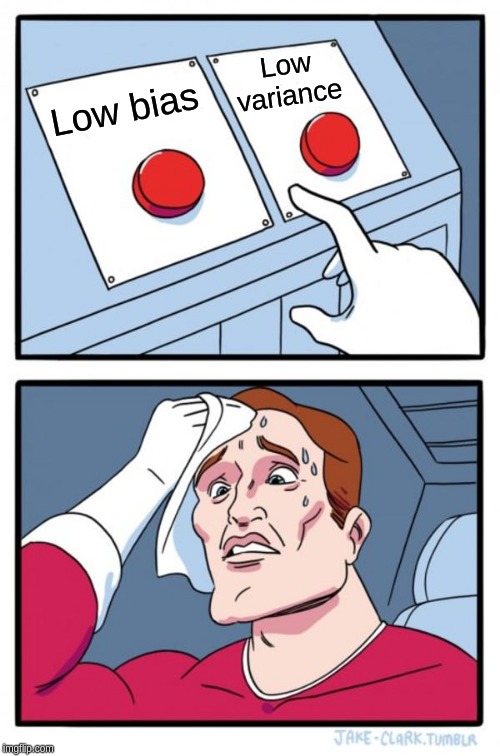
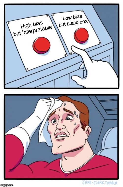
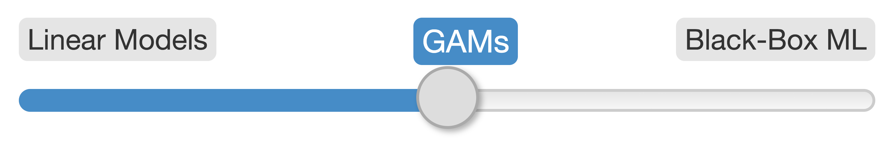
Learning involves trade-offs
The wibbly wobbly stuff — splines
Splines formed from basis functions

Weight basis functions → spline
How do GAMs learn from data?

Choose weights to best fit data
Outputs
Developing methodological approaches
Developing packages to enable model-fitting by other scientists
Training
Simpson (2018) Frontiers in Ecology & Evolution
Pedersen et al (2019) PeerJ
Badly explained stats
Stats profs be like
Badly explained stats
Stats profs be like
Students be like

Master Agreement on Apportionment
12 rivers in AB, SK, MB
Apportionment of inter-provincial river water
Water quality objectives
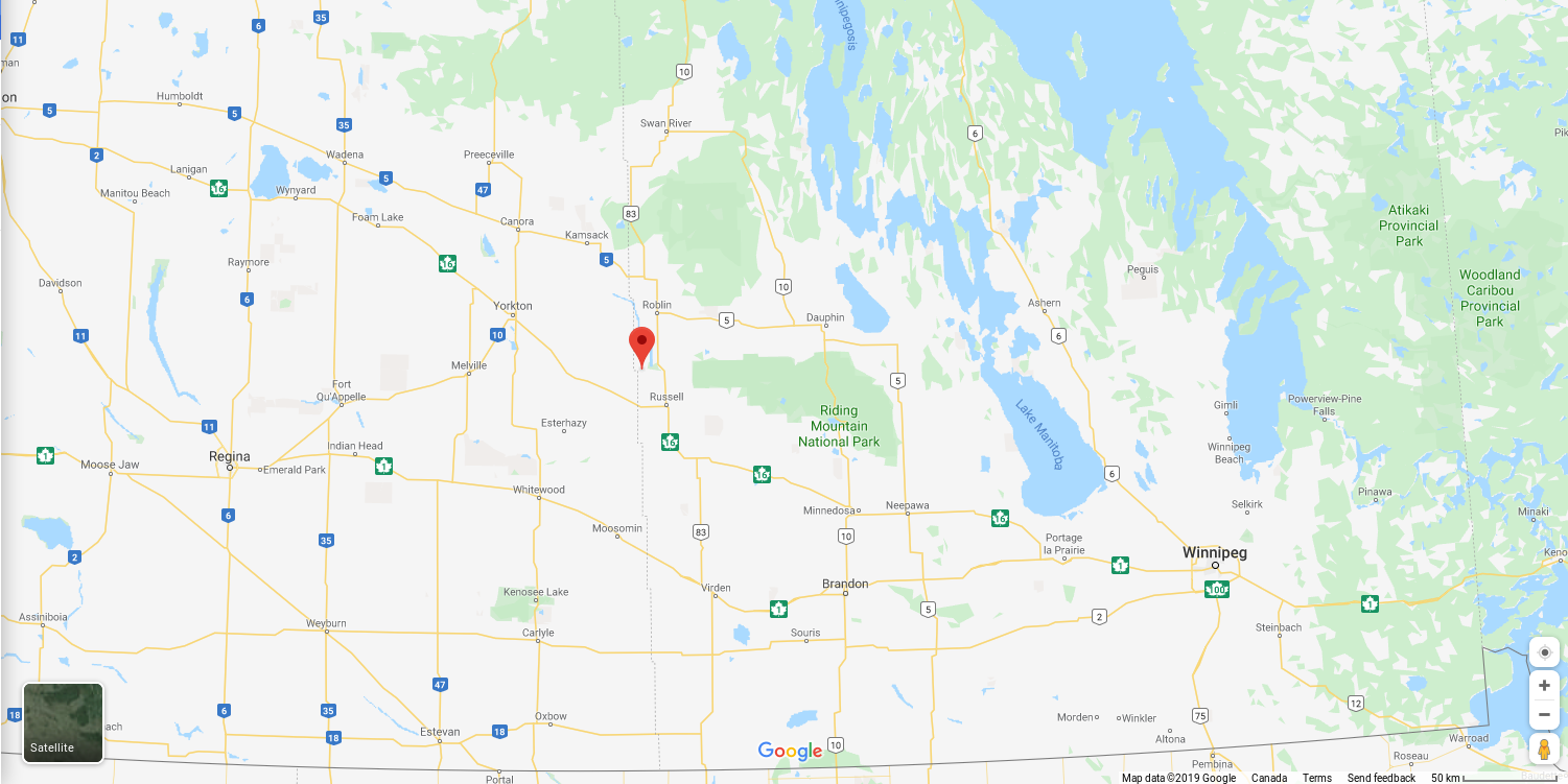
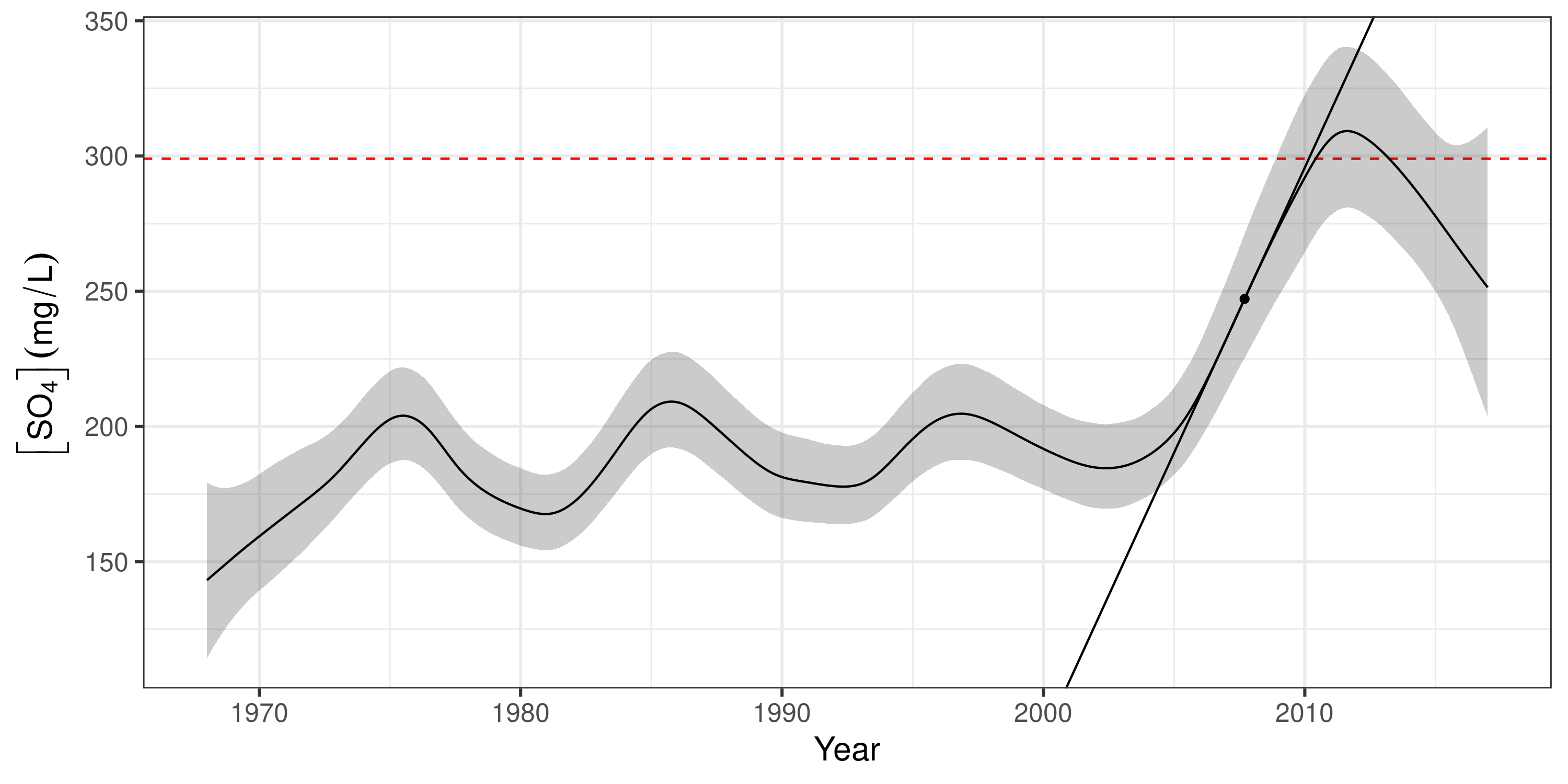
Sulphate in the Assiniboine River
Sulphate ([SO4]) in Assiniboine River near Shellmouth
No significant increases over the years
Keep [SO4] < 299 mg L-1
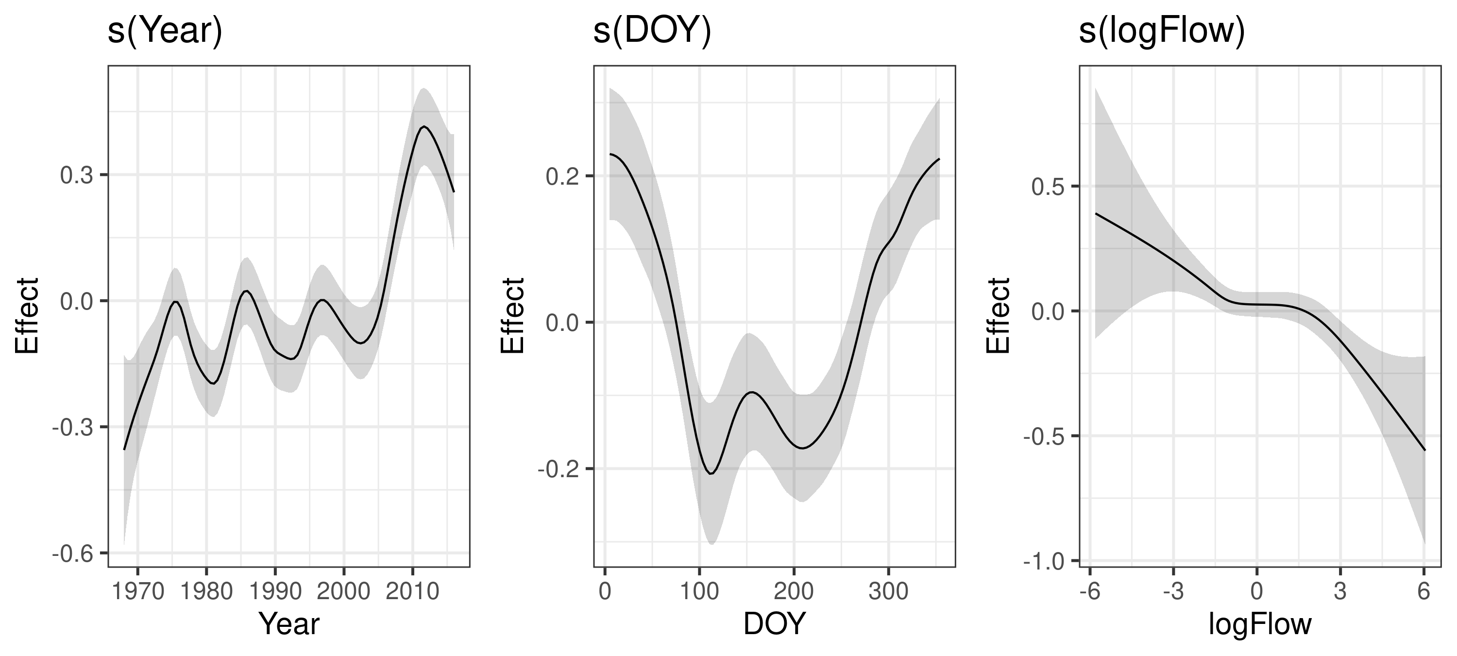
Model structure I
Create a model with year, seasonal, and flow effects
Model structure II
Add interactions between terms
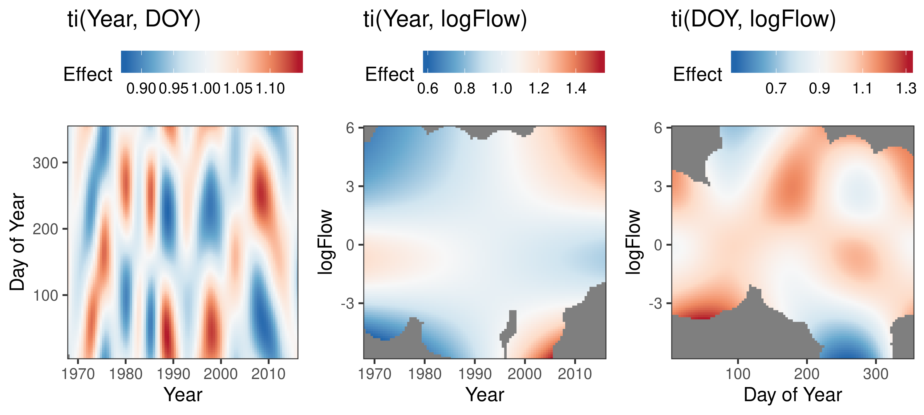
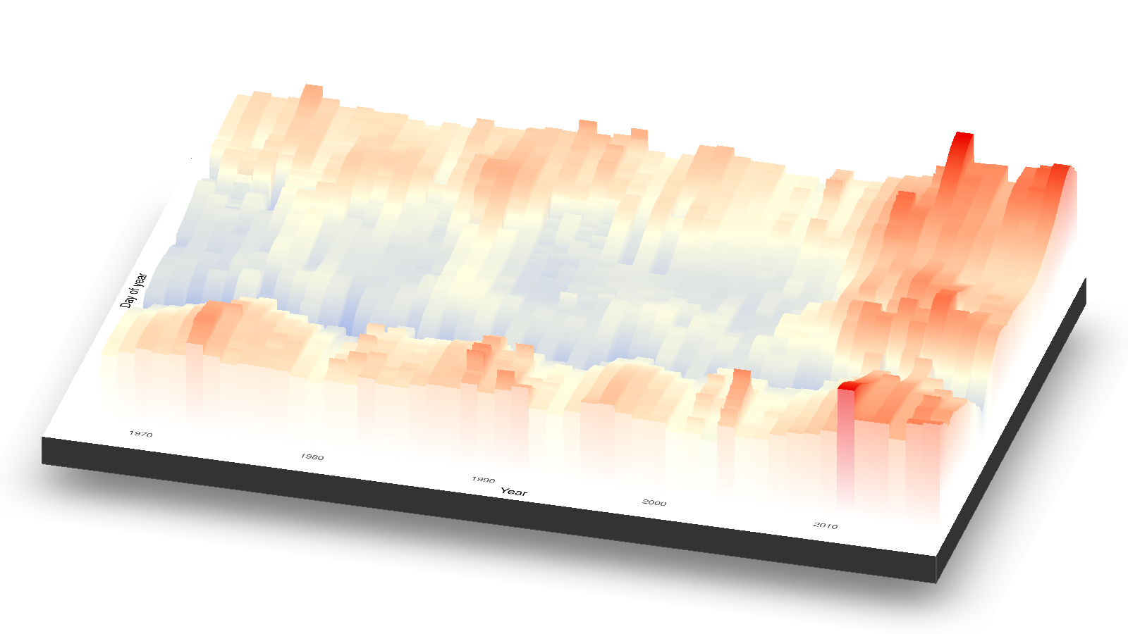
Expected [SO4] over time
Expected [SO4] given log(Flow)
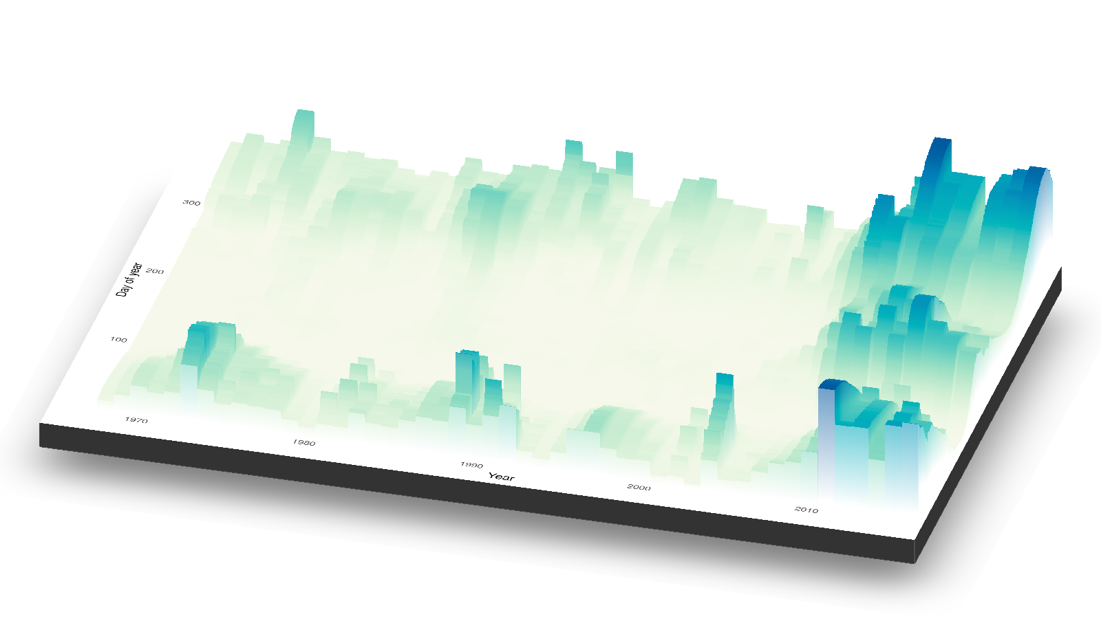
P( [SO4] >299 mg L-1 ) given log(Flow)
Instantaneous rate of change
Identify periods of change
Identify periods of significant change

Multiple time series → HGAM

Annual minimum temperature

Fisher–Tippett–Gnedenko theorem
The maximum of a sample of iid random variables after proper renormalization can only converge in distribution to one of three possible distributions; the Gumbel distribution, the Fréchet distribution, or the Weibull distribution.
Negate the minima

Estimated smooths


Acknowledgements
Funding

![]()
Data
- Prairie Provinces Water Board — Dr. Joanne Sketchell
- Environment and Climate Change Canada & Government of Canada
- Iestyn Woolway and colleagues for archiving the lake surface water data
Slides
- HTML Slide deck bit.ly/bio-wibbly © Simpson, Hinz, Mezzini (2019)

- RMarkdown Source