Decluttering ordination plots part 3: ordipointlabel()

Previously in this series I looked at first the ordilabel() and then orditorp() functions in the vegan package as means to improve labelling in ordination plots. In this the third in the series I take a look at ordipointlabel().

Numerical optimisation algorithms take a problem, such as the optimal placement of labels on an ordination plot, and from a starting point iteratively improve the solution to the problem until it can’t be improved any further. Many optimisation algorithms will only accept a better solution as the next update step in the optimisation. As a result, such algorithms tend not to explore widely the solution space from the starting location and can get stuck in a local optimum because they will only accept better solutions; once you are walking downhill in a particular valley you have to stop at the bottom of that valley if you can only walk downhill, even if a better solution is just over a slight rise.

Simulated annealing (SANN) is a stochastic optimisation algorithm. In simulated annealing, the next step in the optimisation is selected probabilistically from the solution space; better solutions are favoured, but worse solutions can also be accepted. This feature allows simulated annealing to explore the solution space during the early iterations. As iterations proceed, the chance that a worse solution will be accepted as the next step is gradually reduced in a way that akin to the gradual cooling used when annealing in metallurgy to minimise defects in the worked metal. As a result the algorithm gradually focuses in on a good solution. There is still no guarantee that this solution is is the globally best solution but the chances of getting stuck in a poor local optimum are reduced.

ordipointlabel() uses SANN to optimise the difficult problem of locating labels to minimise their overlap in the ordination plot. It is modelled after the pointLabel() function of the maptools package.

As with the previous posts, I’ll illustrate ordipointlabel() through a PCA of the Dutch Dune Meadow data set distributed with vegan. Load the package and the data and fit the PCA. We don’t need a priority variable for this example but will use scaling = 3 throughout

## load vegan and the data
require("vegan")
data(dune)

ord <- rda(dune) ## PCA of Dune data

scl <- 3 ## scaling = 3

ordipointlabel(), as its name suggests, labels points hence the resulting plot will include points (plotting characters) as well as a label for each point. The label can be positioned to the left or right, or above or below the point or at any of the corners (top-left etc). The SANN optimisation has a preference for placing labels above points and a slight penalty against drawing them at the corners. ordipointlabel() will find an optimal positioning for each label minimising label overlap. However it should be noted that there is not guarantee that the solution found will be optimal; a local optima may be encountered rather than a global maximum, but the SANN algorithm can act to reduce the chance of being stuck in a local optima.

ordipointlabel() is a self-contained plotting function hence an entire PCA joint plot can be produced through a single call as follows, with the resulting plot shown below

set.seed(314) ## make reproducible
ordipointlabel(ord, scaling = scl)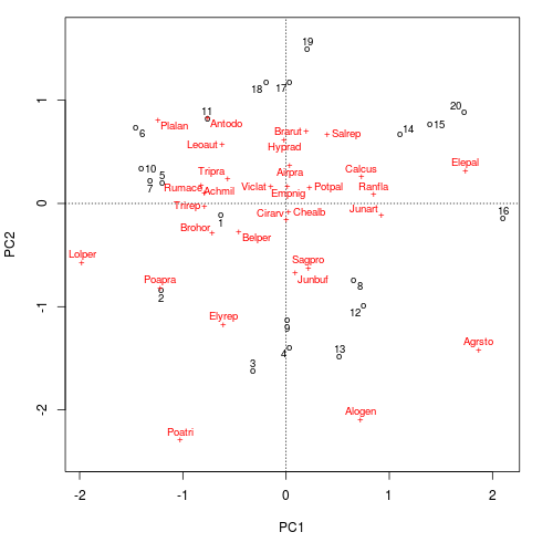

The key feature of the resulting plot that differs from the standard plot() method is that the actual site (sample) and species (variable) scores are marked with a plotting character and that these are then labelled.

Notice that the random number generator is seeded prior to the call to ordipointlabel(); SANN can choose, at random, to move to a worse solution during optimisation and hence to get repeatable results we need to set the random seed. You will also have noticed that the plot doesn’t appear immediately. The SANN optimisation is a slow process and even a simple plot such as the one we just created takes a second or two to optimise on my 18-month old laptop.

By default ordipointlabel() does the following

• PCA axes 1 and 2 are plotted (choices = 1:2)
• both species (variable) and site (sample) scores are drawn (display = c("sites", "species"))
• samples drawn in black, species in red (col = c(1, 2))
• species drawn with a "+", samples with an "o" (pch = c("o", "+"))

ordipointlabel() also has an argument select, which takes a vector indicating which sites (samples) or species (variables) are selected for plotting. This only works when a single set of scores is being drawn (i.e. length(display) == 1). select can be a logical vector indicating which to plot or a numeric vector of indices selecting the scores to plot.

The only other major feature is the ability to add points and labels to an existing plot via the add argument, which defaults to FALSE hence the behaviour we saw earlier.

The object returned by ordipointlabel() is sufficient to recreate the plot without having to re-run the SANN optimisation. A longer example will illustrate this feature

set.seed(42)
plt <- ordipointlabel(ord, choices = c(1,3),
                      col = c("forestgreen", "navy"),
                      pch = 1:2, font = c(1,3), scaling = scl)

plt is now an object of class

> class(plt)
[1] "ordipointlabel" "orditkplot"     "list"

The key class is "ordipointlabel", which has plot() method if you are running a recent development version of vegan (any revision >= 2537). If you’re not, then you won’t see any methods, but see below for a temporary solution.

> methods(class = "ordipointlabel")
[1] plot.ordipointlabel*

   Non-visible functions are asterisked

To illustrate reusing plt and to see how far we’ve come in decluttering the ordination, I conclude by drawing the default PCA plot and the one created in plt.

layout(matrix(1:2, ncol = 2))
op <- par(mar = c(5,4,1,2) + 0.1)
plot(ord, choices = c(1,3), scaling = scl)
plot(plt)
par(op)
layout(1)

The resulting figure is shown below

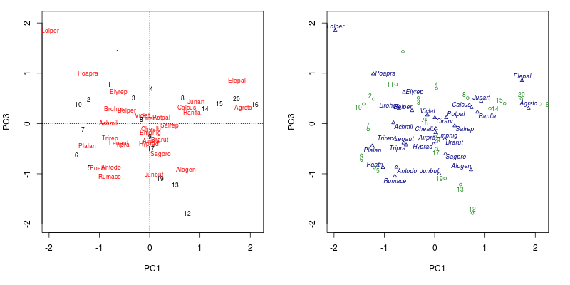
If you are running a version of vegan without the plot.ordipointlabel() method, then you should be able to reproduce the plot by sourcing this version of the function and calling the function directly

## define the plot method locally 
plot.ordipointlabel <- function (x, ...) {
    plot(x$points, pch = x$args$pch, cex = x$args$pcex, col = x$args$pcol,
        bg = x$args$pbg, xlim = x$args$xlim, ylim = x$args$ylim,
        asp = 1, ...)
    font <- attr(x$labels, "font")
    if (is.null(font))
        font <- par("font")
    text(x$labels, rownames(x$labels), cex = x$args$tcex, col = x$args$tcol,
        font = font, ...)
    invisible(x)
}

## draw the plot, calling the new function explicitly
layout(matrix(1:2, ncol = 2))
op <- par(mar = c(5,4,1,2) + 0.1)
plot(ord, choices = c(1,3), scaling = scl)
plot.ordipointlabel(plt)
par(op)
layout(1)

The eagle-eyed among you will have noticed that plt inherited from the class "orditkplot". orditkplot() is an even higher level way to declutter ordination diagrams. orditkplot() uses the tk toolkit and the tcl language distributed with R to implement a rudimentary GUI that allows you to move labels for points around on ordination diagrams and send the object back to R for plotting. I’ll look in more detail at orditkplot() in the next post in this series.

Comments