What's wrong with LOESS for palaeo data?

Gavin Simpson

Locally weighted scatterplot smoothing (LOWESS) or local regression (LOESS) is widely used to highlight “signal” in variables from stratigraphic sequences. It is a user-friendly way of fitting a local model that derives its form from the data themselves rather than having to be specified a priori by the user. There are generally two things that a user has to specify when using LOESS; λ the span or bandwidth of the local window and α the degree of polynomial used in the local regression. Both control the smoothness of the fitted model, with smaller spans and higher degree polynomials giving less-smooth (more-rough) models. Usually it is just the span value that is changed, for expedience.

What can I have possibly against this? What is wrong with using LOESS for palaeo data?

The problem as I see it stems from the way palaeolimnologists choose the LOESS parameters when fitting stratigraphic data. Quite often the default is chosen in whatever software is used. Some people will play around with the span testing out some values until they get a fit that they are happy with. The more statistically savvy palaeoecologist might use a cross-validation (CV) to choose the value of span that provides the best out-of-sample predictions of the observed data. For the latter, generalised cross-validation (GCV) would normally be applied to avoid repeated fitting to each CV fold or subset.

Using the default or the value that gives you a fit that appeals to you is simply not justifiable science. The default may be totally inappropriate for the data to hand and the signal one is expecting. Furthermore, the human brain is great at seeing pattern even where non exists. The smoothness of the fitted LOESS model needs to be chosen to avoid overfitting the observed data. You can’t do that by eye!

CV or GCV should help avoid overfitting the data but importantly can only do this for independent observations in their normal incarnations. Palaeo data are far from independent observations. I’ve blogged before about the problems of smoothing temporally correlated data. Those problems apply just as well to LOESS though they are harder to solve.

Why is this an issue? Well, the reason for fitting LOESS (or any smoother/model) to the stratigraphic data is to show any pattern or trend. With LOESS, what pattern or trend you get is determined by the data and crucially by the parameters chosen for the fit. Once you have the LOESS fit you are going to look at it, ponder what it means, interpret it in light of some other factors, posit a plausible mechanism for its generation. But what if the pattern or trend you’ve lovingly produced isn’t real? What if the features being pondered are statistically indistinguishable from no trend or pattern? LOESS makes it really easy to extract a pattern or trend and because it is a proper stats method it is often taken for granted that the pattern so derived is meaningful.

Consider the example data from the earlier blog post from Kohn et al (2000), where the aim is to uncover the known model from observations drawn from this model with moderate AR(1) noise. The data sample is generated using the following code:

set.seed(321)
n <- 100
time <- 1:n
xt <- time/n
Y <- (1280 * xt^4) * (1- xt)^4
y <- as.numeric(Y + arima.sim(list(ar = 0.3713), n = n))

Several R functions can fit LOESS-like models (e.g. lowess() and loess()in base R but note these two are not the same type of LOESS model). The code chunk and figure below show three fits using different values for the span parameter.

## fit LOESS models
lo1 <- loess(y ~ xt) ## span = 0.75
lo2 <- update(lo1, span = 0.25)
lo3 <- update(lo1, span = 0.5)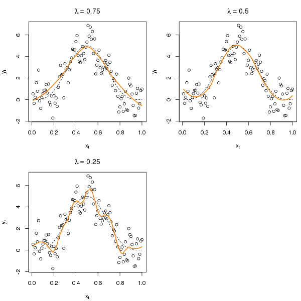

Three LOESS fits to the example data using span = 0.75, 0.25 and 0.5

The plot was produced using

COL <- "darkorange1"
layout(matrix(1:4, nrow = 2))
plot(y ~ xt, xlab = expression(x[t]), ylab = expression(y[t]),
     main = expression(lambda == 0.75))
lines(Y ~ xt, lty = "dashed", lwd = 1)
lines(fitted(lo1) ~ xt, col = COL, lwd = 2)
plot(y ~ xt, xlab = expression(x[t]), ylab = expression(y[t]),
     main = expression(lambda == 0.25))
lines(Y ~ xt, lty = "dashed", lwd = 1)
lines(fitted(lo2) ~ xt, col = COL, lwd = 2)
plot(y ~ xt, xlab = expression(x[t]), ylab = expression(y[t]),
     main = expression(lambda == 0.5))
lines(Y ~ xt, lty = "dashed", lwd = 1)
lines(fitted(lo3) ~ xt, col = COL, lwd = 2)
layout(1)

There is little to choose between \( \lambda \) = 0.75 and \( \lambda \) = 0.5 if we are comparing them with the known model (the dashed line), but suppose we don’t know the true model? The optimal \( \lambda \) according to GCV can be determined using a function modified from a posting to R-Help by Michael Friendly (the original function did more than compute GCV)

loessGCV <- function (x) {
    ## Modified from code by Michael Friendly
    ## http://tolstoy.newcastle.edu.au/R/help/05/11/15899.html
    if (!(inherits(x,"loess"))) stop("Error: argument must be a loess object")
    ## extract values from loess object
    span <- x$pars$span
    n <- x$n
    traceL <- x$trace.hat
    sigma2 <- sum(resid(x)^2) / (n-1)
    gcv  <- n*sigma2 / (n-traceL)^2
    result <- list(span=span, gcv=gcv)
    result
}

The optimize() function can be used to find the value of \( \lambda \) that achieves minimal GCV. A small wrapper function is required to link optimize() with loessGCV()

bestLoess <- function(model, spans = c(.05, .95)) {
    f <- function(span) {
        mod <- update(model, span = span)
        loessGCV(mod)[["gcv"]]
    }
    result <- optimize(f, spans)
    result
}

The optimal \( \lambda \) is chosen using bestLoess(). The optimal \( \lambda \) is about 0.18 with a GCV of around 0.009

> best
$minimum
[1] 0.1813552

$objective
[1] 0.009433405

Our original LOESS model can be updated to use this \( \lambda \)

lo.gcv <- update(lo1, span = best$minimum)

The fit this gives is shown in the figure below

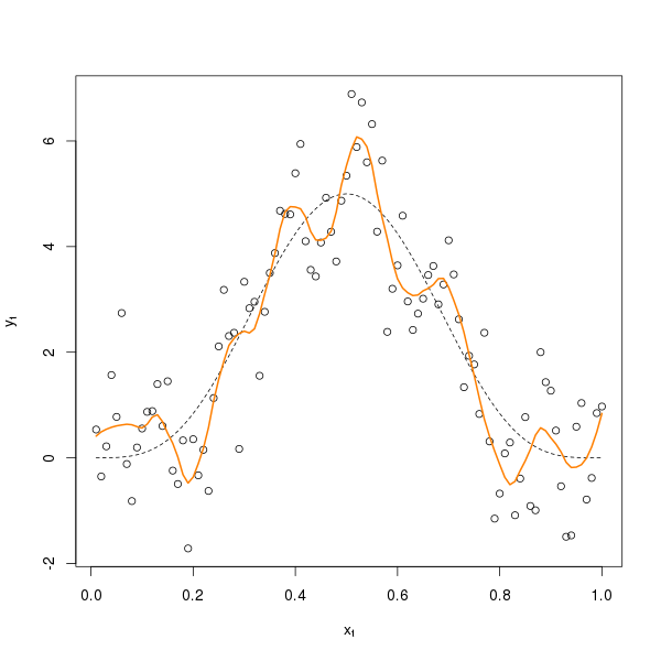
LOESS fit using optimal value of \( \lambda \)

This model clearly overfits; the result of the GCV criterion not knowing that the data are temporally autocorrelated. The whole process assumes that the data are independent and clearly palaeo data often violate this critical assumption. If you didn’t know the real underlying model the average palaeo type would already be penning their next paper on remarkable variation in [INSERT TIME PERIOD] climate from [INSERT SITE]. Yet all that wiggliness, the signal, just isn’t real. Take another sample of data and you would get about the same level of wiggliness but in different places; the signal is just a figment of the sample of data you happen to have collected.

There are solutions to this problem of course; h-block CV has been suggested as a more appropriate means of CV for time series where h observations either side of the target observation are left out from the data used to fit the model to predict the target. There are variations on approach too, as h-block CV tends to over-fit in some situations. I’ll go into this in a bit more detail in a later posting. Be very careful using LOESS for palaeo data!

References

Kohn R., Schimek M.G., Smith M. (2000) Spline and kernel regression for dependent data. In Schimekk M.G. (Ed) (2000) Smoothing and Regression: approaches, computation and application. John Wiley & Sons, Inc.